Vector Databases for RAG
A Deep Dive into What’s Actually Happening Under the Hood

A typical RAG (Retrieval-Augmented Generation) application works in three stages:
you ingest documents by splitting them into chunks and storing their vector embeddings alongside metadata
you retrieve the most semantically relevant chunks at query time by searching for embeddings closest to the query’s embedding, and
you pass those chunks to an LLM to generate a grounded response.
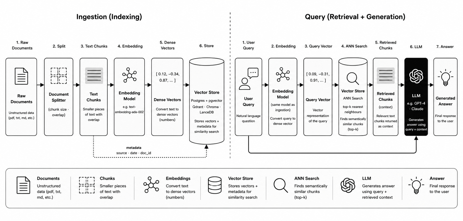
The database sits at the center of this — it stores the embeddings, indexes them for fast nearest-neighbor search, and lets you filter results by metadata like document source, user ID, or date.
For a personal project or small-scale deployment, reaching for Postgres with pgvector is a completely reasonable call: you likely already have Postgres running, adding a vector index is one command, and everything stays in one place. But as soon as your filtering requirements get more demanding — per-user document isolation, selective filters over millions of vectors — the differences between databases start to matter a lot.
This post goes deep on what those differences actually are.
The Filtering Problem
Before diving into each database, it’s worth understanding the core tension that separates them. A real-world vector search isn’t just “find similar vectors” — it’s “find similar vectors within a subset.” You want results filtered by metadata: only this user’s documents, only files from this source, only content from this date range.
This seems like a simple addition. It isn’t.
Vector indexes — HNSW, IVFFlat and metadata indexes — BTree, inverted index are completely separate data structures with no connection between them.
When a query has both a vector similarity condition and a metadata filter, the database has to choose one index to drive the query — it cannot use both simultaneously. This creates a fundamental tension: the vector index finds similar vectors efficiently but knows nothing about your metadata; the metadata index finds matching rows efficiently but knows nothing about vector similarity.
Every database resolves this tension differently. There are three broad strategies:
Post-filtering — use the vector index first to get the top candidates, then apply the metadata filter to the results. The problem: if your filter is selective (only 1% of rows match), the vector index returns candidates that mostly fail the filter. You ask for 10 results and get 2. The database doesn’t warn you — it silently under-delivers.
Pre-filtering — apply the metadata filter first to get all matching rows, then brute-force vector search over that subset. The problem: the vector index is completely bypassed. Fine when the subset is small. Falls apart when the filtered subset is large.
Filtered index traversal — navigate the vector index while skipping nodes that fail the filter, guided by a separate metadata index. Adaptively fall back to brute force when the filter is too selective. This is the right answer — and it’s hard to implement. The vector index was built without knowing your filter condition, so most traversal paths lead through irrelevant nodes. Doing this efficiently requires co-designing the metadata index and the vector index from the start.
With that framing in place, let’s look at each database.
pgvector
pgvector is a Postgres extension — not a separate database, not a separate service.
You install it on an existing Postgres instance, and it adds two new things: a vector column type and HNSW/IVFFlat index types that operate on those columns. For a small project, this is genuinely compelling: vectors, documents, metadata, and all your other relational data live in one Postgres database, and you get transactions, SQL joins, foreign key constraints, backups, and the full Postgres ecosystem for free.
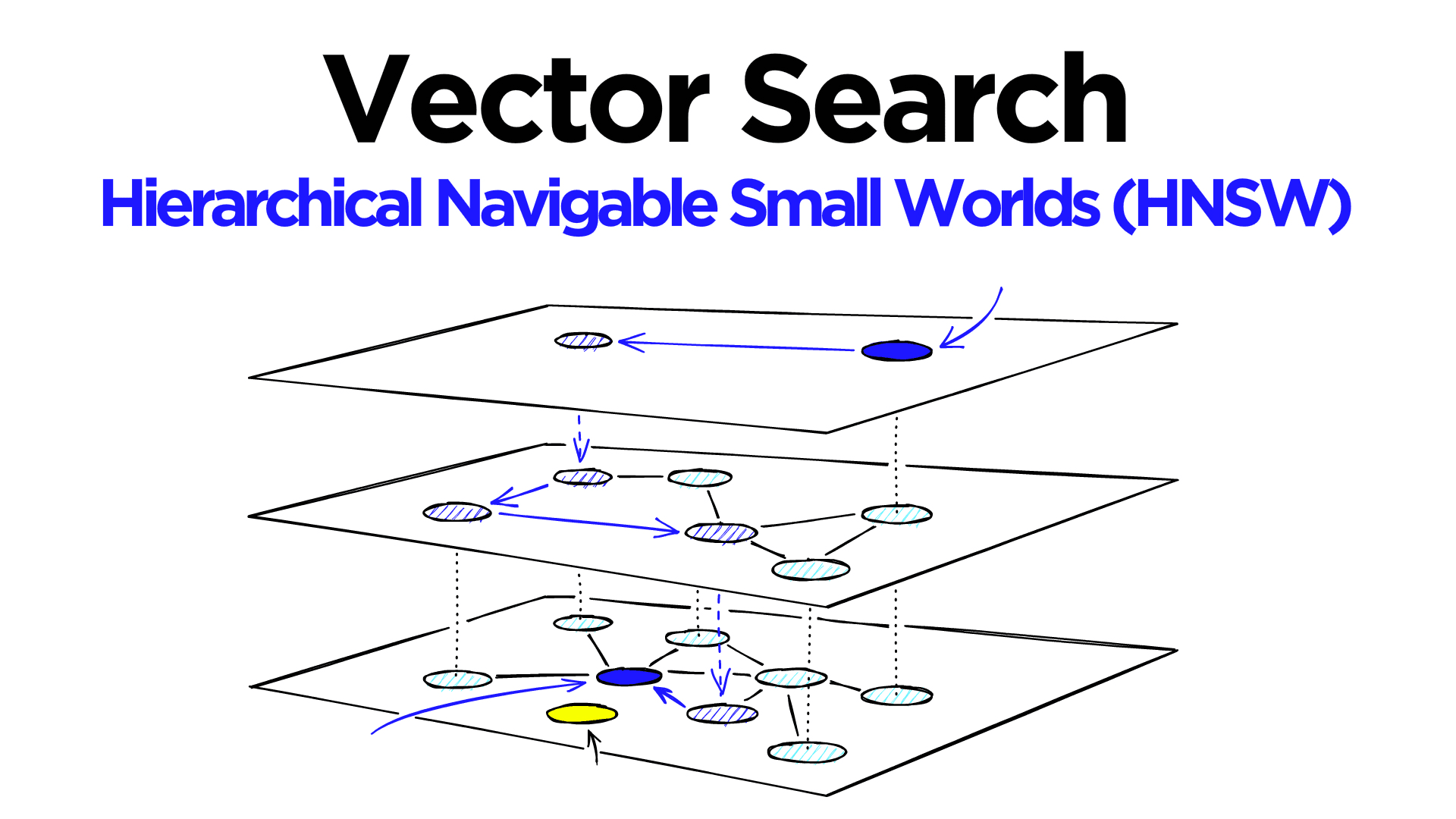
You can watch this video on Youtube if you want to learn a bit more about how HNSW works in a bit more detail.
Adding it is minimal:
CREATE EXTENSION IF NOT EXISTS vector;
ALTER TABLE chunks ADD COLUMN embedding vector(1536);
CREATE INDEX ON chunks USING hnsw (embedding vector_cosine_ops);
That’s it. Your existing Postgres table now has a nearest-neighbor index on the embedding column.
How pgvector handles filtering
Metadata lives in standard Postgres columns (often JSONB). The HNSW index and any metadata index (BTree, GIN) are completely separate structures. When you issue a filtered vector query, the Postgres query planner must pick one index to drive the query.
pgvector defaults to post-filtering: the HNSW index runs first, and the filter is applied to the candidates afterward. For very selective filters, pgvector has an iterative mode that fetches more candidates when the filter removes too many, but this makes query time unpredictable — the database keeps expanding the candidate set until it has enough results or exhausts the index.
A typical query looks like:
SELECT id, content, 1 - (embedding <=> $1) AS similarity
FROM chunks
WHERE user_id = $2
ORDER BY embedding <=> $1
LIMIT 10;
The Postgres planner may choose to drive this via the HNSW index (fast vector search, then filter) or via an index on user_id (fast metadata filter, then brute-force vector scan). With a very selective user_id filter — each user has 0.1% of the total rows — the planner will likely choose the metadata index, and you get brute-force vector search over that user’s rows. With a loose filter (majority of rows pass), the HNSW index gets used and post-filtering works fine.
Where pgvector works well
Pure vector search, no filter: excellent. HNSW index is fully utilised.
Loose filters (filter passes >50% of rows): acceptable. Post-filtering doesn’t lose many results.
Small filtered subsets: fine. Brute force over a few hundred rows is fast.
Where pgvector breaks down
Selective filters (filter passes <5% of rows): recall degrades silently. The HNSW index returns candidates that mostly fail the filter and there aren’t enough left.
Multi-tenancy: filtering by
user_idwhere each user has a small fraction of the data is exactly the worst case for post-filtering.
The operational simplicity — everything in one Postgres database you already run — is a real advantage that’s easy to underestimate. At moderate scale with loose filtering requirements, this is hard to beat.
ChromaDB
ChromaDB is designed for simplicity and local development. It’s the easiest vector database to get running — no infrastructure, no server required in its default embedded mode.
Storage architecture
Collection: “chunks”
  ├── chroma.sqlite3          — all metadata, embedding IDs, collection config
  ├── index/
  │     └── hnsw/            — hnswlib index files (binary graph)
  └── (in memory)            — ID → vector mapping for brute-force filtered search
Chroma uses two completely separate systems: SQLite for metadata and hnswlib (a C++ HNSW implementation) for vector search. In embedded mode, everything runs in the same Python process — no server, no network calls, no configuration.
The hnswlib index
hnswlib is a C++ header-only library that implements HNSW. Chroma wraps it with Python bindings. The index is serialised to disk as binary files and loaded entirely into memory at startup.
This has direct consequences:
First startup after adding many vectors is slow — the entire index loads into RAM
The entire HNSW index must fit in RAM — no memory-mapping, no on-disk access
The index is periodically persisted to disk, not on every write — there’s a crash risk window where metadata (in SQLite) and the HNSW index can diverge
How Chroma handles filtering
Chroma uses pre-filtering exclusively. For any filtered query, it queries SQLite first to get matching IDs, then brute-force searches the vector space for those IDs. The HNSW index is bypassed entirely for any filtered query. Every filtered query is a linear scan over the matching subset, regardless of how large that subset is.
This means:
Filtering correctness: always correct, always complete results. You never get silently under-delivered results.
Filtered queries at scale: with hundreds of thousands of vectors in the filtered subset, brute-force becomes the bottleneck. The HNSW index only helps for completely unfiltered searches.
The SQLite ceiling
Every vector has a corresponding row in SQLite with its ID, collection ID, and metadata (stored as JSON). For filtered queries, Chroma issues a SQLite SELECT to get matching IDs, then searches those IDs in hnswlib. The SQLite database becomes a bottleneck at scale — it’s a single file with write locks, not designed for high-concurrency vector workloads.
Chroma doesn’t pretend to be a production-scale database. SQLite as the metadata backend was a deliberate “keep it simple” choice. It excels at what it’s designed for: getting something working quickly, locally, without infrastructure. The filtering limitation is an acceptable tradeoff for that audience.
Qdrant
Qdrant is a purpose-built vector database written in Rust, designed from scratch with filtering as a first-class requirement. This co-design is what makes its filtering qualitatively better than the alternatives.
Storage architecture
Collection: “chunks”
  ├── Segment 1
  │     ├── vectors.dat       — raw float vectors, memory-mapped
  │     ├── payload.db        — metadata (JSON), stored in RocksDB
  │     ├── hnsw_index/       — HNSW graph files
  │     └── payload_index/    — BTree / inverted indexes per field
  ├── Segment 2
  │     └── (same structure)
  └── ...
Qdrant organises data into collections (equivalent to a table). Within a collection, data is split into segments — self-contained storage units, each with its own HNSW index, vector storage, and payload storage. This segmented architecture is key to several of Qdrant’s properties.
New writes go into a special appendable segment. Periodically, Qdrant merges and optimises segments in the background — compacting small segments into larger ones and rebuilding the HNSW index over the merged data. There’s no “rebuild the index” downtime event; optimisation happens continuously in the background while queries keep running.
How Qdrant handles filtering
At query time, Qdrant builds a filter bitmap — a set of which vector IDs pass the filter condition — using the payload index. During HNSW graph traversal, it only counts nodes in the bitmap as valid candidates. If the filter is very selective, it adaptively switches to brute-force over the filtered subset. This adaptive decision is made at query time based on estimated selectivity.
The payload index and the HNSW index were co-designed to work together. You can’t bolt this onto an existing system cleanly — it’s an architectural consequence of being designed with filtering in mind from day one.
Qdrant’s filtering advantage shows up most in multi-tenancy scenarios. A payload index on user_id means per-user filtering is efficient regardless of how selective the filter is. Whether 50% or 0.1% of vectors match, the adaptive strategy picks the right approach.
Vector storage options
Qdrant gives you explicit control over how vectors are stored — a knob pgvector doesn’t expose at all:
In-memory — the entire vector dataset is loaded into RAM. Fastest queries, limited by available memory.
Memory-mapped — vectors live on disk but are accessed via mmap. The OS manages what’s in RAM. Works for datasets larger than RAM, with some latency when pages aren’t cached.
On-disk — vectors are read from disk on every query. Slowest, but handles very large datasets.
The right default for most production deployments is mmap. Hot vectors (frequently accessed) naturally stay cached by the OS page cache; cold vectors stay on disk. The HNSW graph structure — the edges and pointers — is kept in RAM even in mmap mode, because graph traversal involves many random pointer hops you can’t afford disk reads for.
Quantization
Qdrant supports scalar quantization and product quantization to compress vectors in memory:
Scalar quantization: compress float32 (4 bytes) to int8 (1 byte) — 4x memory reduction, ~1% recall loss
Product quantization: more aggressive compression, ~32x reduction, more recall loss
The compressed vectors are used for the HNSW graph traversal. The original full-precision vectors are kept on disk and used to re-score the final candidates — a two-pass approach that preserves recall while dramatically reducing memory usage. No other database in this comparison handles this as cleanly.
Pinecone
Pinecone is a fully managed cloud vector database. You don’t run it — you call an API. It’s the most production-hardened option and the only one where scaling is someone else’s problem.
Namespaces and metadata filtering
Pinecone introduces two concepts that don’t exist in the other databases: namespaces and managed metadata filtering.
Namespaces are hard partitions at the index level — think of them as completely separate indexes for different tenants or categories. If you put each user’s documents in their own namespace, searching that namespace only touches those vectors. There’s no filtering problem because the data is partitioned before it ever reaches the vector index.
For finer-grained filtering within a namespace, Pinecone uses a proprietary metadata filtering implementation that avoids the recall degradation of post-filtering.
Where it works well
Multi-tenant SaaS applications: namespaces are a first-class concept explicitly designed for this use case.
Production at scale: managed service, no operational burden, automatic scaling.
Filtering correctness and performance: both handled — no silently degraded recall, no brute-force fallbacks at scale.
Where it falls short
Cost: not free, and at scale the pricing is significant.
Vendor lock-in: fully managed means you don’t control your infrastructure or your data’s location.
No local development: you cannot run Pinecone locally. Development and production both hit the cloud API.
Less transparency: proprietary internals mean less visibility into why queries behave a certain way.
LanceDB
LanceDB is the most architecturally distinct of the four. It’s built on Lance — a columnar storage format designed specifically for ML workloads, built on top of Apache Arrow.
Storage architecture
Collection: “chunks”
  └── chunks.lance/
        ├── data/
        │     ├── part-0.lance    — columnar data files (vectors + metadata together)
        │     ├── part-1.lance
        │     └── ...
        ├── _indices/
        │     └── hnsw/           — IVF + HNSW index files
        └── _transactions/        — versioning log
Everything — vectors, metadata, and other columns — lives in the same columnar files. This is fundamentally different from the other databases, where vectors and metadata are stored separately.
The Lance columnar format
Lance stores data in columns rather than rows. For a chunks table with columns id, content, embedding, source, created_at:
Traditional row storage:
  [id1, content1, vec1, source1, date1]
  [id2, content2, vec2, source2, date2]

Lance columnar storage:
  ids:       [id1, id2, id3, ...]
  contents:  [content1, content2, content3, ...]
  embeddings:[vec1, vec2, vec3, ...]
  sources:   [source1, source2, source3, ...]
For vector search, this layout is powerful: you can read only the embeddings column without touching content or source. For filtered search, you can read only the source column to evaluate the filter without loading vectors at all. This makes scan-heavy operations much more cache-efficient.
There are several reasons this matters for ML workloads specifically:
You almost never need all columns at once. A vector search needs embeddings. A filter needs source. Displaying results needs content. These are separate operations that can now each read only what they need.
Compression is dramatically better. Similar values are adjacent — sources might be ["a.txt", "a.txt", "a.txt", "b.txt", ...]. Run-length encoding compresses this to almost nothing. Columnar formats routinely achieve 5-10x compression over row formats on real datasets.
SIMD vectorised computation. Modern CPUs have SIMD (Single Instruction, Multiple Data) instructions that perform the same operation on 8 or 16 values simultaneously. A 256-bit AVX2 register holds 8 float32 values; a 512-bit AVX-512 register holds 16. For cosine similarity between two 384-dimension vectors, SIMD turns 384 multiply-add operations into ~24 SIMD instructions — a real 8–16x speedup on the math. SIMD requires values to be contiguous in memory. With row storage, embeddings for different rows are separated by all the other column data. With columnar storage, all embeddings are adjacent, and the CPU can load and operate on multiple vectors in the same instruction cycle. This is why PyTorch, NumPy, and FAISS are all fast — they store data in columnar/contiguous layouts and exploit SIMD.
Arrow interop. Apache Arrow is an in-memory columnar format — the same layout as Lance on-disk, but in RAM. Pandas, NumPy, PyTorch, and most ML tooling speak Arrow natively. A LanceDB dataset can be converted to a Pandas DataFrame or a PyTorch tensor with zero copying. With Postgres, you’d query, get rows back, and then reshape the data — copying it multiple times.
Versioning
Every write to LanceDB creates a new version — old data is never mutated in place. This gives you:
Time travel — query the database as it was at any past version
Reproducibility — ML experiments can pin to a specific dataset version
Atomic writes — a write either creates a new version or doesn’t; no partial states
This is borrowed from the data lake world (Delta Lake, Apache Iceberg) and is unique among the vector databases here.
The index
LanceDB uses a combination of IVF (for coarse partitioning) and HNSW (for fine search within partitions). The index is disk-native — it doesn’t need to fit in RAM, making LanceDB well-suited for datasets that are large relative to available memory.
The filtering story is better than pgvector and Chroma but not as sophisticated as Qdrant. Because metadata and vectors are in the same columnar files, filtered scans can be more efficient — the columnar layout means reading only relevant columns. But LanceDB still does pre-filtering (scan the filter column, get matching rows, vector search over those rows) rather than Qdrant’s filtered graph traversal.
The embedded / serverless angle
LanceDB runs embedded (in-process, like Chroma) or against object storage (S3, GCS) directly — with no server in between. A LanceDB collection can live in an S3 bucket and be queried directly from a Lambda function. This is the most cloud-native storage model of the four. No database server to run, no connection pool to manage, pay for storage and compute separately.
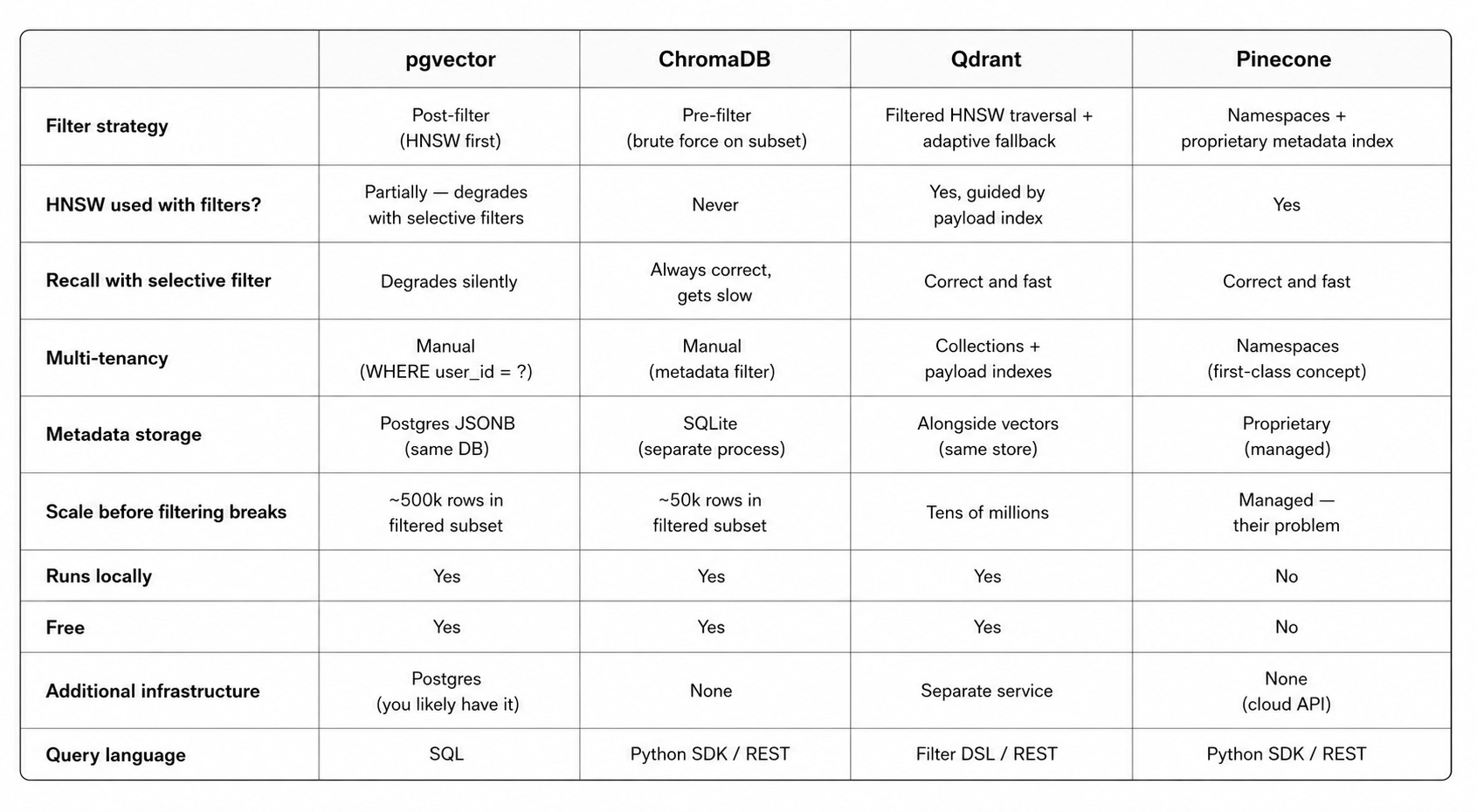
Side-by-Side Comparisons
Filtering and multi-tenancy
Internal architecture
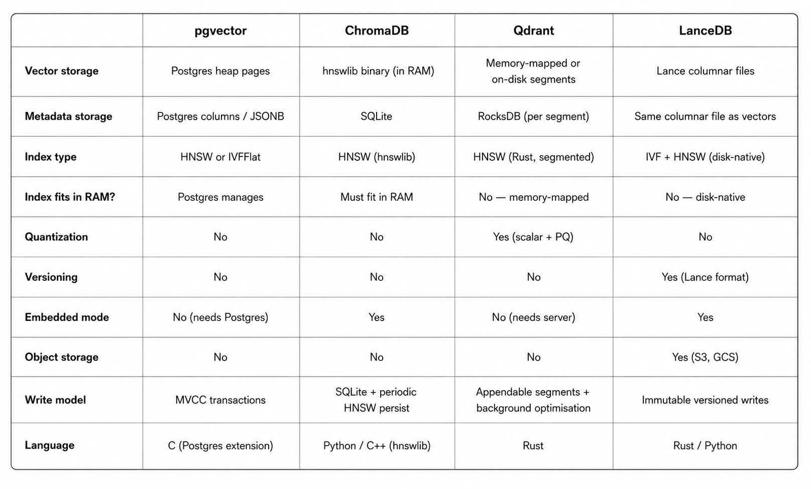
Why the Architectures Differ
The differences between these databases aren’t accidents — they reflect what each system was designed to solve.
pgvector was retrofitted onto Postgres. The vector index was added to an existing general-purpose database with its own query planner and index infrastructure. Combining two indexes is limited by what Postgres’s planner was built to do, which predates vector search entirely.
ChromaDB was built for developer simplicity. SQLite as the metadata backend was a deliberate choice — it’s embedded, zero-config, and works everywhere. Filtering correctness was prioritised over filtering performance because the target user is a developer prototyping locally, not an engineer running millions of queries.
Qdrant was built for production vector search with filtering as a core requirement. The payload index and HNSW index were co-designed. This is why Qdrant’s filtering is qualitatively better — it’s not a bolt-on, it’s foundational.
Pinecone was built for multi-tenant SaaS applications. Namespaces exist because their target customer is a startup building a product for many end users who need per-user isolation from day one. The managed service model reflects that their target customer wants to outsource infrastructure, not run databases.
LanceDB was built for ML workloads at large scale, inheriting design philosophy from the data lake world. Columnar storage and versioning are foundational, not afterthoughts — because the target user is running offline evaluation pipelines, large static corpora, or hybrid analytical and vector workloads.
The filtering problem is a microcosm of a broader pattern in database design: general-purpose systems get retrofitted with new capabilities, while purpose-built systems design those capabilities in from the start. pgvector is Postgres with vectors added. Chroma is an HNSW library with a metadata store added. Qdrant was built as a vector database with filtering in mind. The quality of the filtering experience reflects which approach each system took.
This doesn’t mean purpose-built always wins — it means there’s a real tradeoff between integration simplicity (pgvector: everything in one place) and capability (Qdrant: designed for the hard cases). The right choice depends on which tradeoff matters more for your specific system.
Choosing the Right One
You’re building a prototype or internal tool with one user: pgvector or Chroma. Zero extra infrastructure, simple to reason about, easy to swap out later.
You need filtered search and your filtered subsets are large: Qdrant. The payload index + filtered HNSW traversal is the right architecture for this case.
You’re building a multi-tenant product (each user has their own documents): Qdrant (self-hosted, free) or Pinecone (managed, paid). pgvector and Chroma will degrade.
You’re at scale and want someone else to operate the database: Pinecone. The managed model removes operational burden at the cost of vendor lock-in and price.
You want everything in one database, SQL joins, and you don’t have selective filters: pgvector. The operational simplicity of keeping everything in Postgres is a real advantage that’s easy to underestimate.
Your dataset is very large relative to RAM, you want versioning and reproducibility, or you’re running offline ML evaluation pipelines: LanceDB. The disk-native index, columnar storage, Arrow interop, and versioning are genuine advantages for this workload — and the embedded or object-storage deployment model removes the operational burden of running a server.
You’re building a hybrid system — vector search alongside complex aggregations, analytical queries, or column-scan-heavy workloads: LanceDB or Qdrant, depending on whether you need the analytical query patterns (LanceDB) or the best filtered ANN performance (Qdrant).
The correct approach is to start with pgvector (simple, correct, integrated), understand the tradeoffs clearly, and know when to migrate.
If your system is architected around a pluggable storage abstraction — a VectorStore interface that all retrieval code goes through — then migration is a one-file change rather than a rewrite of your retrieval and generation layers.
The architecture decision isn’t permanent; the cost of getting it wrong is proportional to how tightly coupled your application is to the specific database you chose.
This article was originally published on My Medium Blog.